 Make a Profit & Loss Balance Sheet table.
 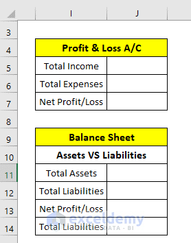 Add an extra table for the Category Name and Category Type.
 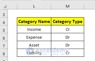 Read More: How to Make a Forecasting Balance Sheet in Excel
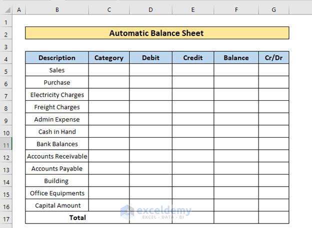
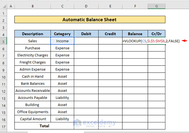
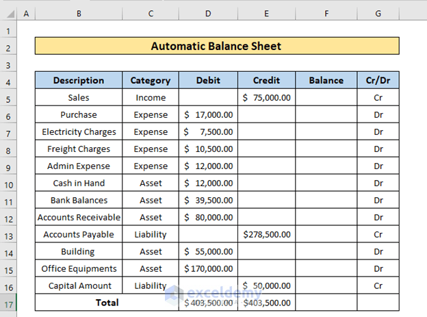
We need to create a balance sheet table. The table can be like the following, which includes columns Category, Debit, Credit, Balance, and Cr/Dr. In the Category, we will define the type of our input, which will help to separate debit and credit. Make a Profit & Loss Balance Sheet table. Add an extra table for the Category Name and Category Type. Read More: How to Make a Forecasting Balance Sheet in Excel
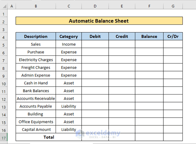
In the table, provide the Category first. Sales are income for the business, and purchases and bills are expenses. Cash in hand and bank balance are assets for the business. Accounts payable and capital amount are liabilities. We categorized them accordingly.
C5 is the lookup value,
$L$5:$M$8 is the table array,
2 is the column index number and
FALSE is a range lookup for an exact match.
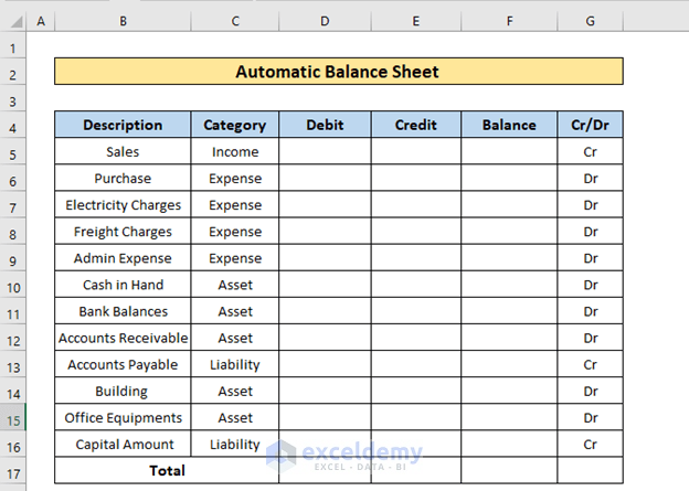
We can see the debit or credit type for each category.
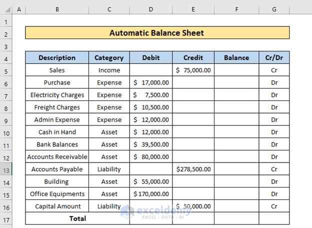
Credit is money flowing out of the account, so we inserted Income and Liability in the Credit column. In contrast, Expense and Asset are inserted in the Debit column because debit means money flowing into the account.
Calculate and verify our balance.
We want the sum of debits below the Debit column in cell D17.
Enter the following formula in the cell:
=SUM(D5:D16)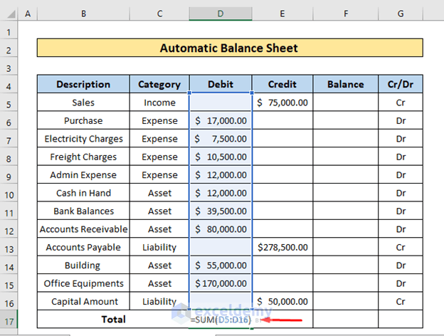
Press ENTER and use the Fill Handle to copy the formula to the cell beside.
We can see the sum of all debits and credits in the bottom cells, which match.
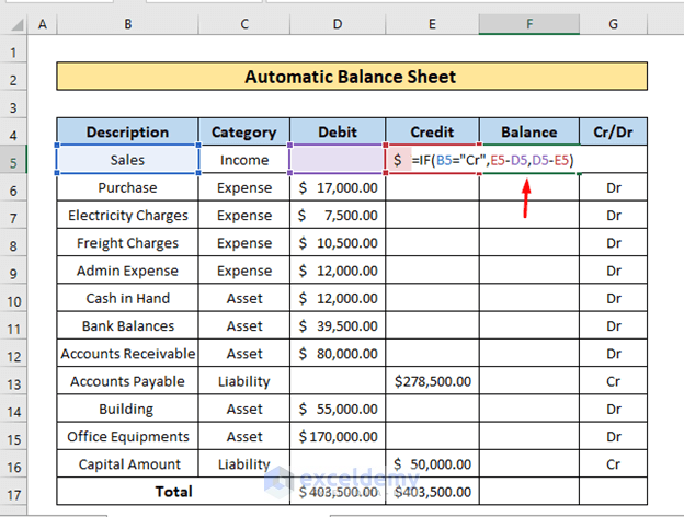
We will make the balance for each input.
Here, IF is an Excel function,
B5=”Cr” is the criteria,
E5-D5 is the result if the criteria match,
D5-E5 is the result if the criteria don’t match.
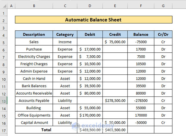
We can see the balance for each input. Credit is shown as a negative value, and Debit as a positive value.
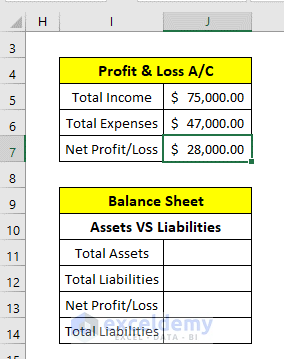
Calculate profit and loss, as well as asset and liability.
Here, we have taken the subtraction value of the 2 SUMIF function.
$C$5:$C$16 is the criteria range,
“Income” is the criteria
E5:E16 is the sum range.
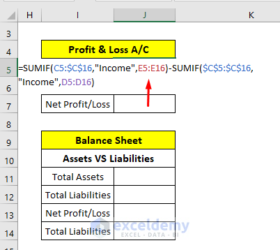
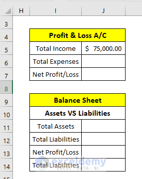
We can see the total income.
Calculate the total expense.
Here, we used the subtraction value from 2 SUMIF functions.
$C$5:$C$16 is the criteria range,
“Expense” is the criteria
D5:D16 is the sum range.
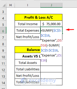
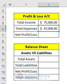
We can see the total expense now.
Here, we have used the subtraction value of 2 cells J5 and J6.
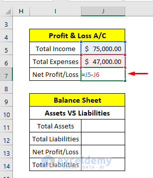
We can see the net profit or loss.
The formula is similar to the formula used previously.
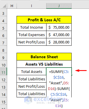
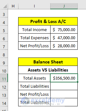
We can see the total assets in the cell.
The formula is similar to the previously used formula.
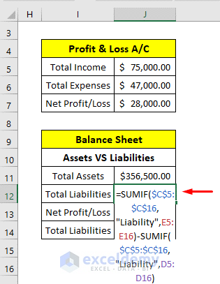
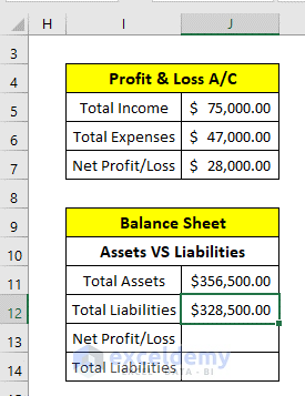
We can see the total liabilities in the cell.
We used the subtraction value of cells J11 and J12.
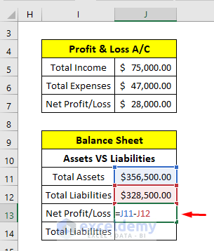
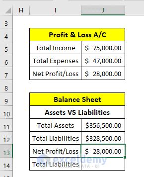
We can see the net profit/loss here, the same as the profit calculated from total income and expenses.
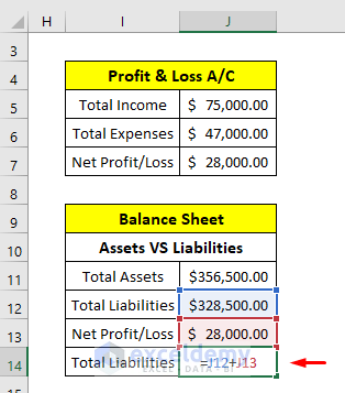
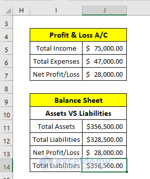
We will see total liabilities there.
Download the Practice Workbook
You can download the practice workbook from here.
Automatic Balance Sheet.xlsx